Living away from your hometown implies being on the move and travelling back and forth. In this personal data project, I decided to visualize the travels I have done in 2019 so far (until September) completely in R, making a code that can be reused, just by putting more travels in the excel file, and manually assigning coordinates to travel segments.

First step as always is to load the needed libraries.

library(tidyverse)
library(readxl)
library(sf) 
library(rnaturalearth)
library(rnaturalearthdata) # To get map of world
library(gganimate)
library(ggimage)
library(jechaveR)
library(magick)

A simple function that will be useful later in the analysis. Remember if you need to copy paste it at least one time create a function instead!

prefix_to_columns <- function(df,prefix){
  df_temp <- df
  colnames(df_temp) <- paste0(prefix,colnames(df_temp))
  df_temp
}

Data

Data is collected manually based on my calendar bookings. Bus, ferry, planes and long distance trains have been included in this analysis.

travels <- read_xlsx("data/travels_2019/travels_2019.xlsx")

#World data example: #https://www.r-spatial.org/r/2018/10/25/ggplot2-sf.html
world <- ne_countries(scale = "medium", returnclass = "sf")

Planes have been added with IATA airport code, so I will use the following internet resource

airports_raw <- read_csv("https://datahub.io/core/airport-codes/r/airport-codes.csv")
airports <- airports_raw %>% 
  select(iata_code,municipality,iso_country,coordinates) %>% 
  filter(!is.na(iata_code))

First let’s check that there are no duplicates in the airports database

travel_sites <- c(travels$from,travels$to) %>% 
  unique()

airports %>% 
  group_by(iata_code) %>% 
  summarize(n = n()) %>% 
  filter(n > 1) %>% 
  filter(iata_code %in% travel_sites) #Check for the sites that we are interested to get the data.

## # A tibble: 1 x 2
##   iata_code     n
##   <chr>     <int>
## 1 MUC           2

We can see that Munich airport has duplicated entries in the database. Let’s first erase this from the data frame.

airports %>% filter(iata_code == "MUC")

## # A tibble: 2 x 4
##   iata_code municipality iso_country coordinates              
##   <chr>     <chr>        <chr>       <chr>                    
## 1 MUC       Munich       DE          11.7861, 48.353802       
## 2 MUC       Munich       DE          11.69029999, 48.137798309

airports <- airports %>% filter(coordinates != "11.69029999, 48.137798309")

Then make a join to get the coordinates from the airport database.

from <- prefix_to_columns(airports,"from_")
to <- prefix_to_columns(airports,"to_")

travels_coord <- travels %>% left_join(from,by = c("from" = "from_iata_code")) %>% 
  left_join(to,by = c("to" = "to_iata_code"))

We still have some values missing as not all the trips are from-to an airport

coord_na <- travels_coord %>% 
  filter(is.na(from_coordinates) | is.na(to_coordinates)) %>% 
  select(from,to) 

data_missing_places <- c(coord_na$from,coord_na$to) %>% unique()

data_missing_places

## [1] "Helsinki"        "Tallinn"         "Tampere"         "Rauma"          
## [5] "Aranda de duero" "Pori"            "Madrid"

Fill missing data manually

complementary_info <- tribble(
  ~site,~municipality,~iso_country,~coordinates,
  "Tallinn","Tallinn","EE","24.7666636, 59.43999824",
  "Helsinki", "Helsinki", "FI", "24.945831, 60.192059",
  "Tampere", "Tampere" , "FI", "23.78712, 61.49911",
  "Rauma", "Rauma", "FI", "21.51127, 61.12724",
  "Aranda de duero", "Aranda de duero","ES", "-3.6892, 41.67041",
  "Pori", "Pori", "FI", "21.78333, 61.48333",
  "Madrid", "Madrid", "ES", "-3.70256, 40.4165",
  "Porvoo", "Porvoo", "FI", "25.66507, 60.39233"
  )

from_2 <- prefix_to_columns(complementary_info,"from_")
to_2 <- prefix_to_columns(complementary_info,"to_")

travels_coord_missing <- travels %>% 
   filter(from %in% data_missing_places & to %in% data_missing_places) %>% 
  left_join(from_2, by = c("from" = "from_site")) %>% 
  left_join(to_2, by = c("to" = "to_site"))

Bind rows from two tables to complete the data.

travels_all <- rbind(travels_coord_missing,
  travels_coord %>%  filter(!is.na(from_coordinates) & !is.na(to_coordinates))
  )

Geodata

We need to proceed with the points and lines that will be shown in the visualization

travel_clean <- travels_all %>% 
  separate(from_coordinates, sep = ",",into = c("from_lat","from_lon"),convert = TRUE) %>% 
  separate(to_coordinates, sep = ",", into = c("to_lat","to_lon"), convert = TRUE) 

With the clean data we can plot the travels with geom_curve()

  ggplot() +
  geom_sf(data = world) +
  coord_sf(xlim = c(-10,35),ylim = c(35,70),expand = FALSE) +
  geom_curve(data = travel_clean,
    aes(x = from_lat, y = from_lon,xend = to_lat, yend = to_lon,color = type), curvature = -0.2) +
  theme_jechave() %+replace%
  theme(panel.grid.major = element_blank(),
    axis.text = element_blank(),
    axis.title = element_blank())

#ggsave("output/travel_geom_curves.jpg",dpi = 600)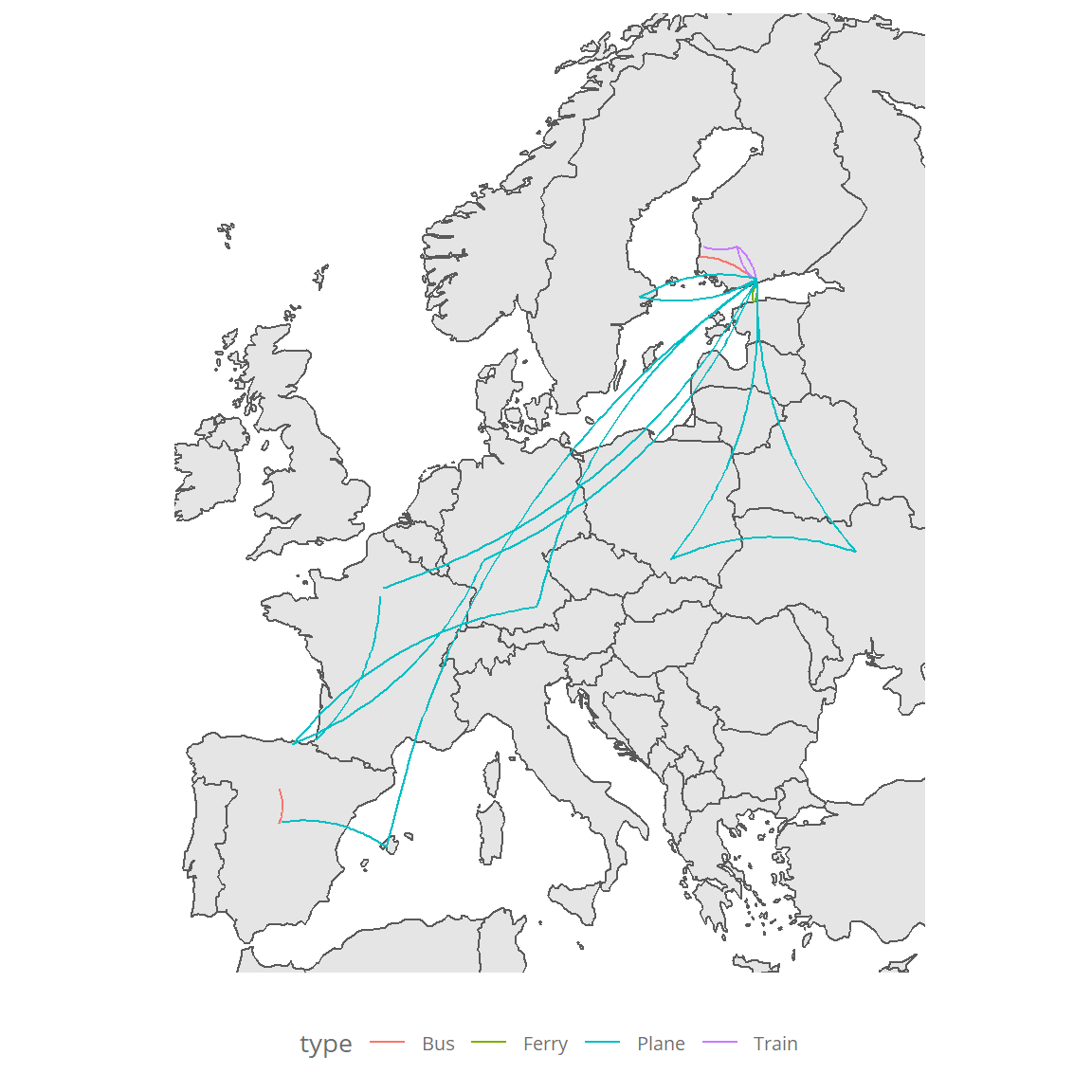

Data transformation

To get the gganimate package to work we need to use the transition. For that purpose we will need to take the starting and end point and create a sequence of intermediate points with the function seq()

subset_df <- travel_clean[1,]
  df <- tibble(
    x = seq(subset_df$from_lat,subset_df$to_lat,length.out = 20),
    y = seq(subset_df$from_lon,subset_df$to_lon,length.out = 20)
  )
 test_plot <- ggplot() +
  geom_line(data = df,aes(x, y)) +
  transition_reveal(x)
test_animate <- animate(test_plot,nframes = 5)

 test_animate
# anim_save("output/linemoving.gif",test_animate)

For the animation, I will use the ggimage package and icons from ionicons for the different types of travel.

unique(travel_clean$type)

## [1] "Ferry" "Train" "Bus"   "Plane"

travel_icons <- tribble(
  ~type,~URL,
  "Plane","https://unpkg.com/ionicons@5.0.0/dist/svg/airplane-outline.svg",
  "Ferry","https://unpkg.com/ionicons@5.0.0/dist/svg/boat-outline.svg",
  "Train","https://unpkg.com/ionicons@5.0.0/dist/svg/train-outline.svg",
  "Bus","https://unpkg.com/ionicons@5.0.0/dist/svg/bus-outline.svg")
travel_clean <- travel_clean %>% left_join(travel_icons,by = c("type" = "type")) 

By plotting with ggnamiate the travel with a test flight, we get the following animation

df <- tibble(x = seq(-2.9,11.78,length.out = 10), y = seq(43.30,48.35,length.out = 10),icon = "https://unpkg.com/ionicons@5.0.0/dist/svg/airplane-outline.svg") 
    # Plots
    p1 <- ggplot() + 
        geom_image(data = df, aes(x, y,image = icon)) + 
        geom_line(data = df, aes(x, y),size = 2,alpha = 0.05) +
        transition_reveal(x) +
        labs(title = "geom_line() with transition_reveal(x)")
    p1anim <- animate(p1, nframes = 5)  
    p1anim
    anim_save("output/withoutmap.gif",p1anim)

We can also add the European map as before, note that the order of the geoms will impact of what goes on top of what. That is the reason why the geom_sf and coord_sf go first.

p2 <- ggplot() + 
  geom_sf(data = world) +
  coord_sf(xlim = c(-10,35),ylim = c(35,70),expand = FALSE) + 
 #coord_sf(xlim = c(-10,35),ylim = c(35,55),expand = FALSE) + #For export to twitter
  geom_image(data = df, aes(x, y,image = icon)) + 
  geom_line(data = df, aes(x, y),size = 2,alpha = 0.15) +
  transition_reveal(x) +
  labs(title = "Bilbao - Munich") +
    theme_jechave() %+replace%
  theme(panel.grid.major = element_blank(),
    axis.text = element_blank(),
    axis.title = element_blank())

p2anim <- animate(p2,nframes = 25)
p2anim 

anim_save("output/BIO-MUC.gif",p2anim)

Next step is to create a function to create the visualization for each of the segments. And then thanks to the function purrr::walk we can create a loop to create each of the gifs of the travels, together with their own icon and date

animate_segment <- function(df,segment_num){
  subset_df <- df[segment_num,]
  icon <- subset_df$URL
  day <- subset_df$day
  df_temp <- tibble(
    x = seq(subset_df$from_lat,subset_df$to_lat,length.out = 20),
    y = seq(subset_df$from_lon,subset_df$to_lon,length.out = 20)
  )

 p1 <- ggplot() + 
  geom_sf(data = world) +
  coord_sf(xlim = c(-10,35),ylim = c(35,70),expand = FALSE) + 
 geom_image(data = df_temp, aes(x, y),image = icon) + 
  geom_line(data = df_temp, aes(x, y),size = 2,alpha = 0.15) +
 transition_reveal(ifelse(subset_df$from_lat < subset_df$to_lat,x,-x)) +
  #transition_reveal(-x) +
   labs(title = paste0(day),
     subtitle = paste0(subset_df$from,"-",subset_df$to)) +
      theme_jechave() %+replace%
  theme(panel.grid.major = element_blank(),
    axis.text = element_blank(),
    axis.title = element_blank())
 #Needed for cases where goes negatively in the animation
 if (subset_df$from_lat < subset_df$to_lat) {
   p2 <- p1 + transition_reveal(x)
 }else{
   p2 <- p1 + transition_reveal(-x)
 }
 
output_path <- paste0("output/partial_gifs/","segment_",day,"_",segment_num + 10,subset_df$from,subset_df$to,".gif")
p2anim <- animate(p2,nframes = 25)
p2anim
anim_save(output_path,p2anim) 
}
#Run function for all rows. Will save in folder all segments
walk(1:NROW(travel_clean),~animate_segment(travel_clean,.x))

Last step is to take all the segments and put them into one gif