Although a bit reluctant first about availability and number of stations, this summer I decided to purchase a seasonal pass (costs 30 €) of Helsinki City bikes. As I have been living in a town outside Helsinki, the bikes have proved to be a great means of transportation for short distances where I would have otherwise needed to buy a rather costly transport ticket.
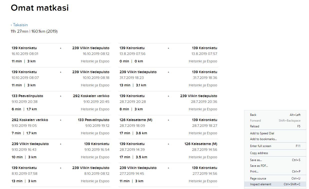
HSL webpage offers the possibility to see the basic information of the travels done with the city bikes.
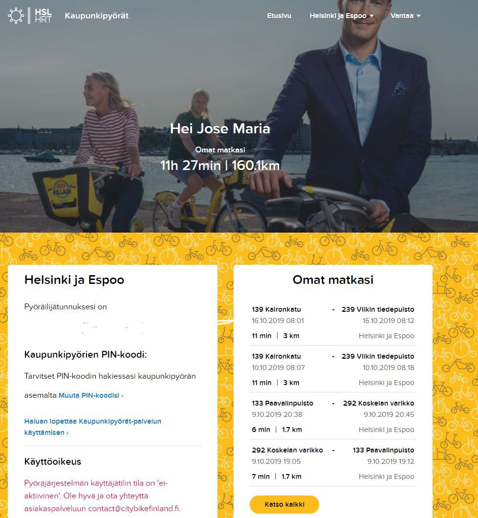
The page also shows some basic data about the different trips. However due to a lack of possibility to download the data, an easy option in order to get the data into a tabular form is web scraping.
So let’s dive into web scraping with R!
Web scrapping step by step
In order to simplify the scrapping since we need to sign in, first step is to go to the HSL city bike webpage https://kaupunkipyorat.hsl.fi/en and downloading the page locally as HTML.
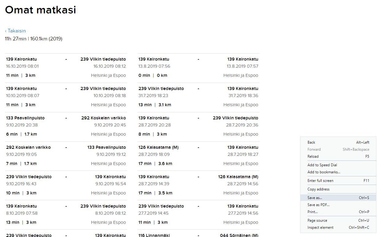
Then we need to go to the page where all travel segments are shown by clicking Katso Kaikki (show all)
First step is to click right mouse button inside the webpage and click save as
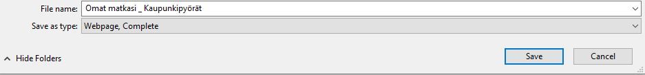
Just save the complete webpage into your project folder
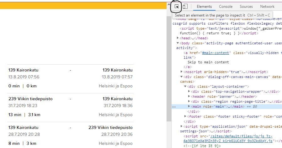
Next step is to Inspect the page elements (this can be done in the actual webpage, or also in the downloaded page).
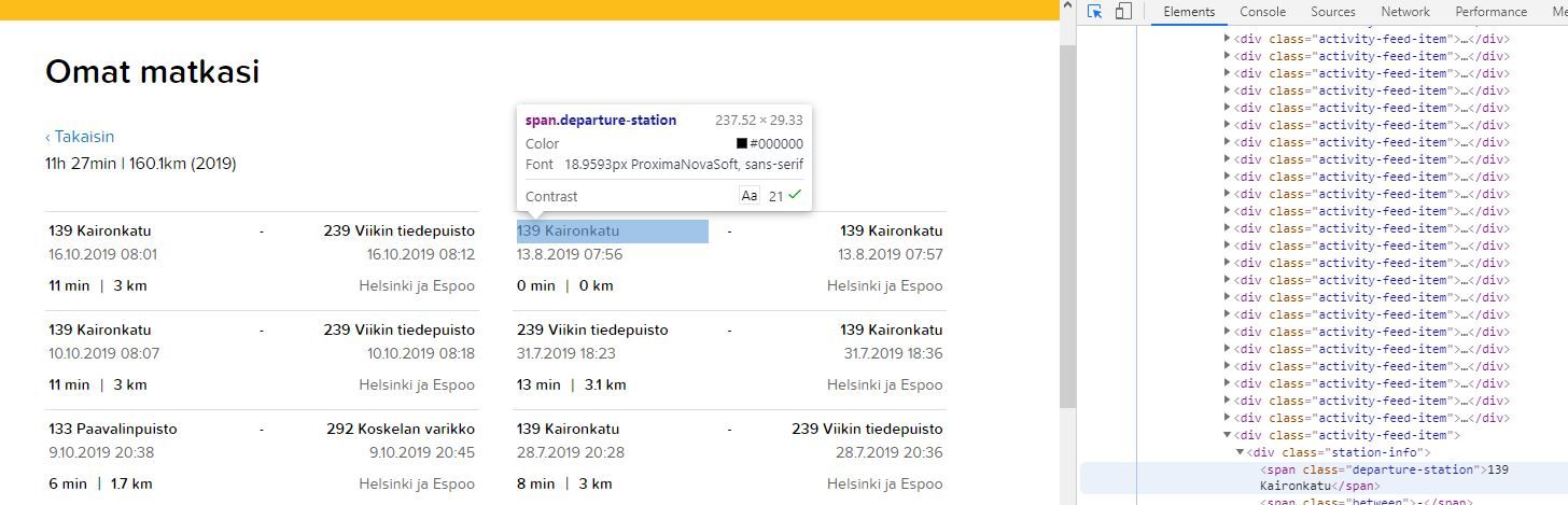
Now we can see some of the code of the webpage, good! But we only need certain parts. So next step is to click the button to select elements, or use the shorcut (Ctrl + Shift + C).
Now every time we hover something in the webpage, it shows parts of its code. As an example, the departure station
Final step is to get the selector for that specific element. We can do that by right mouse click button in the code part related to that element, then we choose Copy -> Copy selector
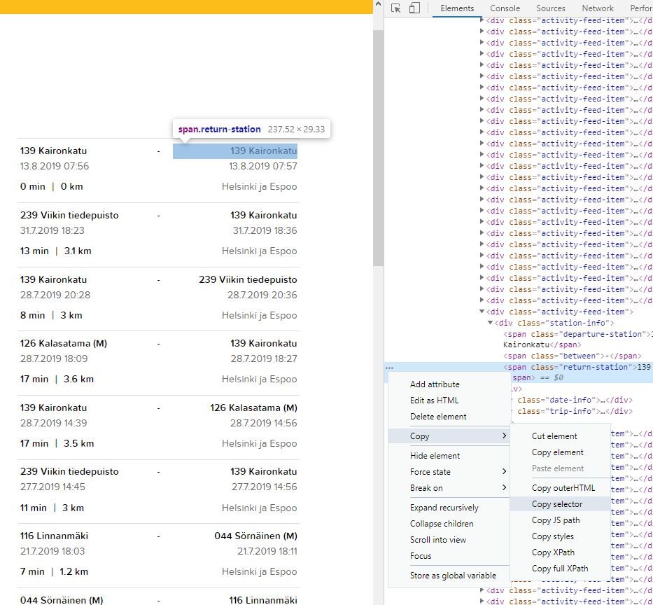
From there we get the following selector for that specific element:
‘#activity-feed > div > div:nth-child(31) > div.station-info > span.return-station’
However we are interested in getting all the similar pieces of text, in this case departure-station. For that we can delete the part :nth-child(31), thus getting the whole list.
We need to do this for all the relevant points of data we are interested on scrapping. Once we have those we can start with getting the info we are interested in.
We will use read_html() from xml2 package and html_nodes() and html_text() from rvest package. Here is the list of all the packages used:
#Scrapping
library(rvest)
library(xml2)
library(jsonlite)
#Data transformation
library(tidyverse)
library(lubridate)
library(glue)
#API calls to HSL
library(ghql) #devtools::install_github("ropensci/ghql")
#Spatial data and maps
library(googlePolylines)
library(sf)
library(ggmap)
library(osmdata)
#Nice table formatting
library(kableExtra)
#personal library
library(jechaveR)
First step is reading the html page.
webpage <- read_html(here::here("static","data","citybikes","bike_routes.html"))Then we will create a named vector with the element selectors.Note that here the selectors are shorter, since in the next step we will be pasting the selector initial part that is repeated in all of the selectors.
selectors <- c(departure_station = "station-info > span.departure-station",
  return_station = "station-info > span.return-station",
  departure_time = "date-info > span.departure-date",
  return_time = "date-info >  span.return-date",
  duration = "trip-info > span.duration",
  distance = "trip-info > span.covered-distance")
Finally, we will loop over all the selectors to read those specific nodes and convert them into text. Column names are defined by the names of the vector.
df_raw <- map_dfc(selectors,~html_nodes(webpage,paste0( "#activity-feed > div > div > div.",.x)) %>%
    html_text(),
  .id = names(.x))
Data transformation
When data scraping is over, now we need to clean the data into something usable for the analysis including station ID numbers and getting numbers for duration and distance. Trips starting and ending in same station are excluded since they are “false rides”.
df <- df_raw %>%
  mutate(departure_time = dmy_hm(departure_time),
    arrival_time = dmy_hm(return_time),
    duration_min = parse_number(duration),
    distance_km = parse_number(distance),
    dep_station_id = str_sub(departure_station,1,3),
    arr_station_id = str_sub(return_station,1,3)) %>%
  filter(dep_station_id != arr_station_id)
In order to get the coordinates of the stops we will make a data_frame with the unique departure-arrival combinations.
stops_unique <- df %>%
  select(dep_station_id,arr_station_id) %>%
  unique()
Coordinates of bike stations can be found in https://www.hsl.fi/en/opendata Helsinki and Vantaa are separated, so rbind will be used to get data of all stations.
all_stations_raw <- read_csv(here::here("static","data","citybikes","HKI_bikestations.csv")) %>%
  rbind(read_csv(here::here("static","data","citybikes","Vantaa_bikestations.csv")))

all_stations <- all_stations_raw %>%
  select(ID,x,y)
Finally, we join the departure station ID with the coordinates, followed by doing the same with the arrival station. This provides us a data.frame with the travels and coordinates for arrival and departure. Which will be used to feed the API and get the route and estimated times.
df_with_coord <- df %>%
  left_join(all_stations,by = c("dep_station_id" = "ID")) %>%
  left_join(all_stations,by = c("arr_station_id" = "ID"),suffix = c("_dep_","_arr_"))
Talking API
Next step is to use an API to get estimated times between directions as well as route details.
HSL offers a graphql API environment to fetch data from. ropensci offers a package to do API calls from R, this are the steps needed to follow:
Initialize client
path <- "https://api.digitransit.fi/routing/v1/routers/hsl/index/graphql"
client <- GraphqlClient$new(
  url = path
)
Make a Query class object
qry <- Query$new()Query function
route_query <- function(from_lat,from_lon,to_lat,to_lon){
  #Generate random ID for the query
 query_hash <- stringi::stri_rand_strings(1,5)
  qry$query(query_hash,glue::glue('
{
  plan(
    from: {lat: <<from_lat>>, lon: <<from_lon>>}
    to: {lat: <<to_lat>>, lon: <<to_lon>>}
    numItineraries: 1
    transportModes: [{mode: BICYCLE}]
  ){
    itineraries {
      legs {
        mode
        duration
        distance
        legGeometry {
          points
        }
      }
    }
  }
}
  ',.open = "<<",
    .close = ">>"))
#Always ghet the last response from the queries
response <- client$exec(qry$queries[[length(qry$queries)]])
#Convert the response to more readable format
result <- fromJSON(response,flatten = TRUE) %>%
  data.frame()
#Filter routes, to take just the longest single trip. (Avoids considering walking few meters)
result[[1]][[1]] %>%
  filter(mode == "BICYCLE") %>%
  filter(distance == max(distance))
}
#Example query
route_query(60.15978,24.91842,60.18204,24.92756)
Once query function is tested and working, we will again use the map family to pass coordinated arguments into the query and arrange them into a data frame.
routes_df <- pmap_dfr(list(df_with_coord$y_dep_,df_with_coord$x_dep_,
  df_with_coord$y_arr_,df_with_coord$x_arr_),route_query)

write_csv2(routes_df,"output/routes_data_HSL_API.csv")
Saving the output, to avoid repeating the API calls in the future.
Data wrangling and geometries
The API returns a handy googlePolylines text string to define the route. This needs to be converted into points.
routes_df <- routes_df %>%
  mutate(duration_min = duration/60,
    distance_km = distance/1000) %>%
  select(duration_min_HSL = duration_min,
    distance_km_HSL = distance_km,
    polyline = legGeometry.points)

points_all <- map_dfr(routes_df$polyline,~decode(.x) %>% as.data.frame(),.id = "trip")
For handling easier, SF will be used and a table with each route and the containing LINESTRING, which is very easy to plot with geom_sf()
linestrings <- points_all %>%
  mutate(point_order = row_number()) %>%
  st_as_sf(coords = c("lon","lat")) %>%
  sf::st_set_crs(4326) %>%
  group_by(trip) %>%
  summarize(n = n(),do_union = FALSE) %>%
  st_cast("LINESTRING")
Final wranglings are combining the data from the webpage and API, together with the newly created linestring table.
all_data_df <- cbind(df_with_coord,routes_df) %>%
  mutate(time_diff = duration_min_HSL - duration_min,
    dist_diff = distance_km_HSL - distance_km,
    trip_num = as.character(row_number()) )

all_data_sf <- linestrings %>%
  left_join(all_data_df,by = c("trip" = "trip_num"))
Simple data exploration
With the data ready and some simple dplyr, it is easy to find the longest bike ride. According to the API, it took 27 minutes more than needed to complete the ride. This was due to a distraction on the way, there was a flea market in the area.
all_data_df %>%
  filter(duration_min == max(duration_min)) %>%
  select(departure_station,return_station,departure_time,time_diff,dist_diff) %>%
  kable() %>%
kable_styling() | departure_station | return_station | departure_time | time_diff | dist_diff |
|---|---|---|---|---|
| 141 Intiankatu | 137 Arabian kauppakeskus | 2019-05-25 11:52:00 | -27.05 | -1.353054 |
In general I have been riding faster than the time defined by the HSL API, which might mean I was taking shortcuts from roads without designated biking lane, or then the speed defined in the API is a safe assumption and rather slow.
ggplot(all_data_sf) +
  geom_jitter(mapping = aes(duration_min,duration_min_HSL)) +
  geom_abline(intercept = 0, slope = 1,color = "red",linetype = "dashed") +
   geom_text(aes(x = 6.5,y = 18,label = "Same route",vjust = 0.5),
    family = "Open Sans",color = "#6d6d6d",size = 3.5)  +
    geom_curve( mapping = aes(x = 11,y = 14.5,xend = 8,yend = 18),
    arrow = arrow(length = unit(0.07, "inch"),ends = "first"),
    size = 0.4, color = "#6d6d6d",curvature = 0.3) +
  theme_jechave() +
  labs(x = "Trip duration (min)",
    y = "Trip estimation HSL (min)",
    title = "Do I ride fast?",
    subtitle = "Above red dotted line, trips riding faster than estimation")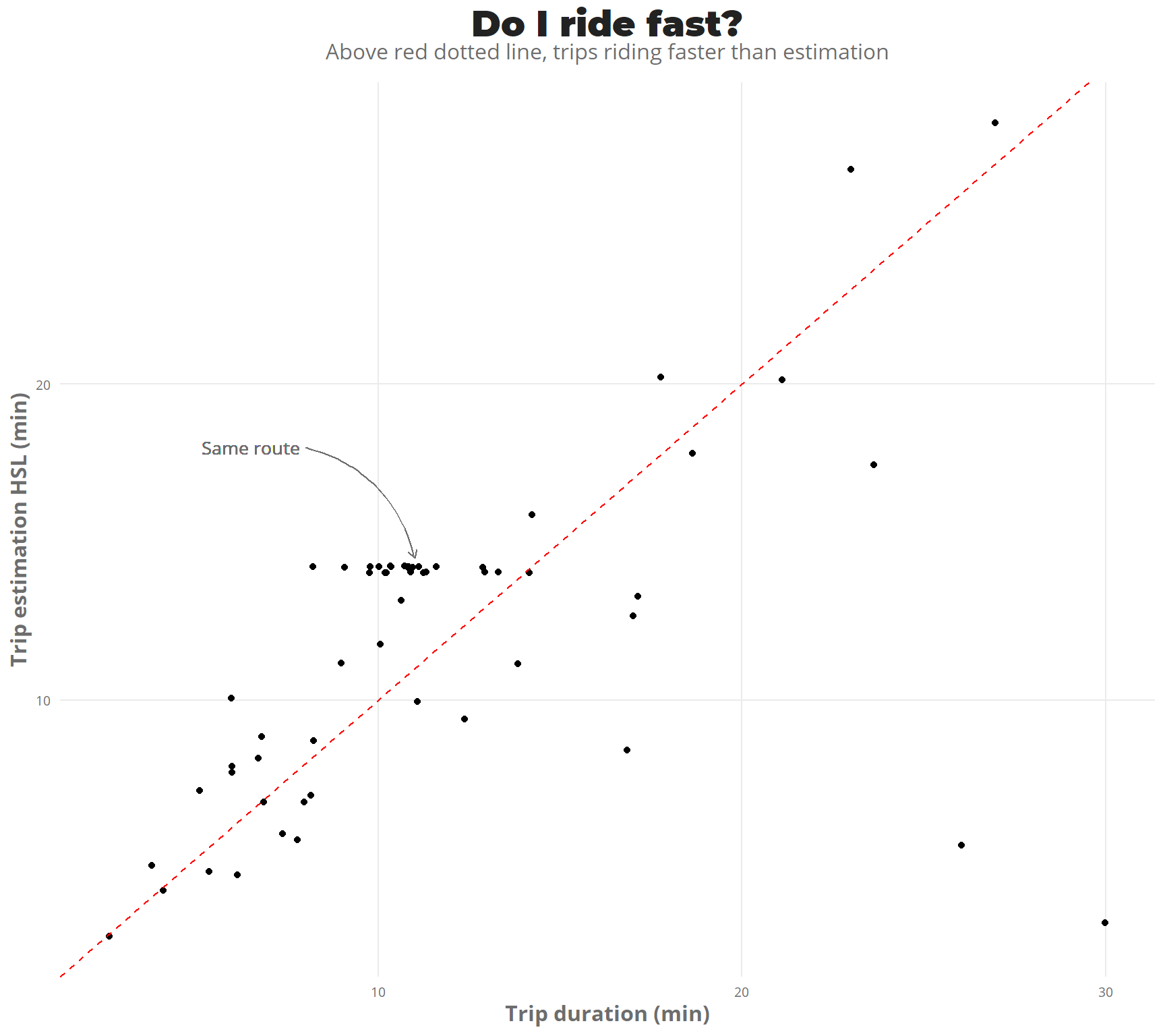
In the plot it can be seen that there is a group of points gathered horizontally, these correspond to the same route done in different days. From Viikki to Arabianranta. Let’s calculate some simple statistics for these trips.
all_data_df %>%
  filter(dep_station_id %in% c("139","239"),
    arr_station_id %in% c("139","239")) %>%
  mutate(direction = case_when(dep_station_id == "139" ~ "Arabianranta -> Viikki",
    TRUE ~ "Viikki -> Arabianranta")) %>%
  group_by(direction) %>%
  summarize(trips = n(),
    mean_duration = mean(duration_min),
    max_duration = max(duration_min),
    min_duration = min(duration_min)) %>%
  kable() %>%
kable_styling() | direction | trips | mean_duration | max_duration | min_duration |
|---|---|---|---|---|
| Arabianranta -> Viikki | 15 | 10.60000000 | 13 | 8 |
| Viikki -> Arabianranta | 9 | 11.44444444 | 14 | 10 |
The trip from Arabianranta to Viikki was mainly to catch the bus, which could explain the shorter durations (fear of missing the bus).
Visualizing all the routes
To finalize, a map visualization where all the routes done with bike are shown. I have used snapbox package to work on top of mapbox and use my own map styling.
Plotting everything together for final result
library(snapbox)
library(sf)
library(ggplot2)
 linestrings_3857 <- st_transform(linestrings, 3857)
area <- st_bbox(
  c(xmin = 24.85, ymin = 60.149, xmax = 25.05, ymax = 60.23),
  crs = 4326
)

map_base <- ggplot() +
  layer_mapbox(area, scale_ratio = 0.5,
    map_style = "mapbox://styles/kutteb/ck9h39xng0png1iqyyvmqchpb",
    mapbox_api_access_token = keyring::key_get("mapbox_token",keyring = "jechaveR"))

map_base +
  coord_sf(crs = st_crs(3857)) +
  geom_sf(data = linestrings_3857,color = alpha("#FED100",0.5),size = 0.75, inherit.aes = FALSE) +
theme_jechave() %+replace%
  theme(panel.grid.major = element_blank(),
    axis.text = element_blank(),
    axis.title = element_blank()) +
  labs(title = "Itineraries in Helsinki City bikes",
    subtitle = "Summer 2019, data from HSL")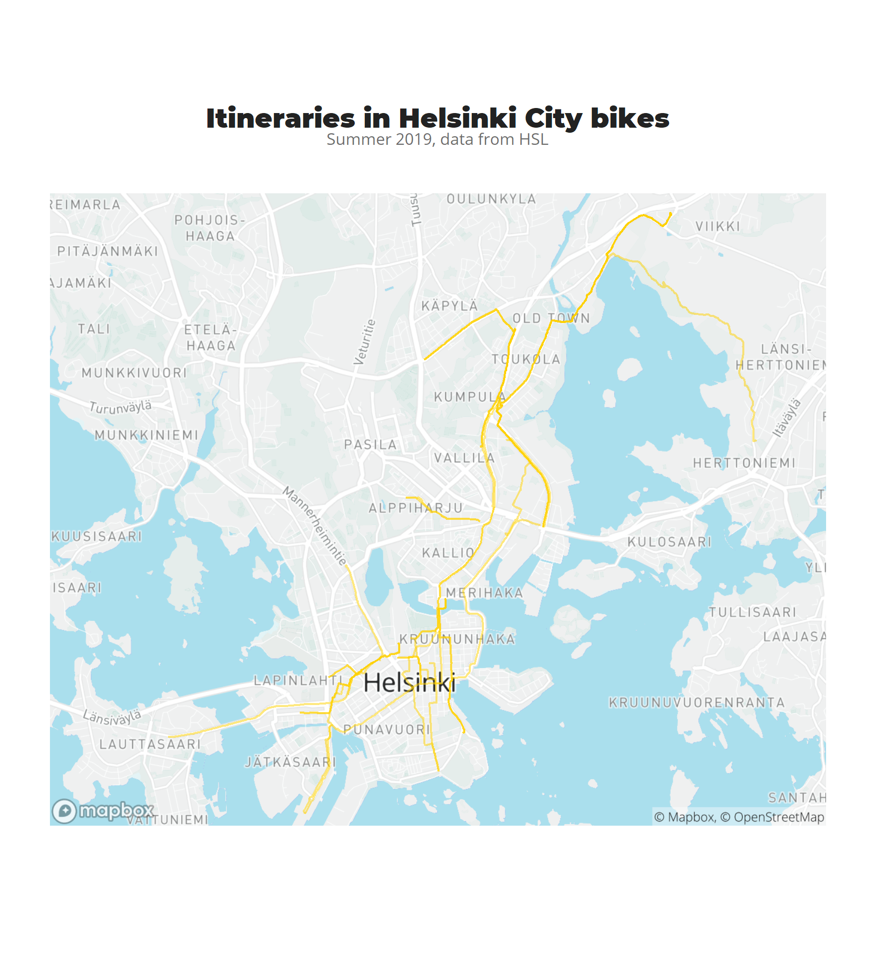
ggsave("citybike_2019_itineraries.png",dpi = 900)Conclusion: In this post we have done some web scrapping, created a personalized function that does API calls and put everything on a map to visualize the usage of the city bikes during the summer season in Helsinki. This has been my story of how I fell in love with those bikes . Cannot wait to see those yellow bikes again on the city.